Cache Memory Simulator

INTRODUCTION

The memory hierarchy consists of multiple memory references such as, CPU registers, L1-L3 Cache, Physical Memory, and Virtual Memory. In class, we covered Cache memory in depth, therefore, to ensure that we truly understand the concept, we will be implementing a Cache Memory Simulator that behaves exactly like a Cache memory component. The simulator will need to read an address file and output the number of simulated addresses, Cache hits, and final hit ratio. Furthermore, we will need to graph the Cache miss rates for all Cache memory parameters. The simulator will be programmed using Python and the graphs will be plotted using Excel.

DESIGN/ARCHITECTURE/ALGORITHM DESCRIPTION

MEMORY HEIRARCHY:

Computer memory typically consists of 4 kinds of memory: CPU registers, Levels 1-3 Cache, Primary Memory, and Secondary Memory (Figure 1). CPU registers are small amounts of high-speed memory that can quickly be accessed by the processor since they are contained within the CPU itself. The following memory component is the Cache memory, which is also located within the CPU, but further away to the processor than the registers. It is a temporary storage area that makes retrieving data from the Primary Memory more efficient. Primary Memory, also known as Main Memory or Physical Space, is the next volatile component in the hierarchy and is where programs and data are kept when the processor is actively using them. The programs and data are copied from the Secondary Memory which allow the CPU to interact with them. The furthest away component from the processor is the non-volatile Secondary Memory, also known as Disk Memory or Virtual Space. This component has the largest amount of storage space; however, it cannot be immediately accessed by the CPU and requires the desired data to be copied over to the Primary Memory first.

Figure 1: Kinds of Computer Memory.

Overall, the further away the memory component is from the CPU, the slower it is going to be. But in contrast, the closer the memory component is to the CPU, the smaller in size that is going to be. Figure 2 simply describes the computer memory hierarchy.

Figure 2: Computer Memory Hierarchy Pyramid.

CACHE MEMORY:

Cache Memory is the second closest memory layer to the processor and serves a purpose of increasing data retrieval performance by reducing the need of accessing the slower storage layers. Typically, there are 3 types of Cache Memory: Level 1 (L1), Level 2 (L2), and Level 3 (L3) Cache. L1 Cache is a small amount of memory that is within the CPU that typically ranges around 64 KB. Each processor core will have it’s own L1 Cache for both Instructions (I-Cache) and Data (D-Cache). L2 Cache can either be contained inside or outside of the CPU and has a typical memory range of 256 KB. Each processor core can have their own L2 Cache or share one with other cores. L2 Cache is slower than L1 Cache. L3 Cache is used to enhance the performance of L1 and L2 Cache. It is located outside of the CPU and typically has a range of 4 MB. Although L3 Cache is slower than the lower two levels of Cache, it is faster than the Main Memory. Figure 3 shows an example of Cache memory for a quad-core processor.

Figure 3: Cache Memory for a Quad-Core Processor.

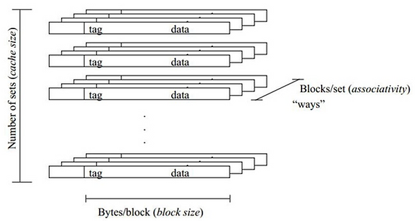
A typical Cache has 3 dimensions and is organized by Cache size, block size, and associativity. A representation of the Cache organization can be seen in Figure 4. To determine the number of lines within the Cache, we take the Cache memory size and divide it by the line size. Note that the line size is equal to block size of the Main memory. If the associativity is direct, designated Main memory blocks will only be mapped to one Cache line. If the associativity is k-way, then there will be k number of lines per set in the Cache. The designated Main memory blocks will be able to map to any of those lines within the set. For Full associativity, the Main memory blocks will be able to map to any line in the Cache memory. The Tag will let us know which Main memory block is stored in the Cache memory line.

Figure 4: Cache Memory Organization.

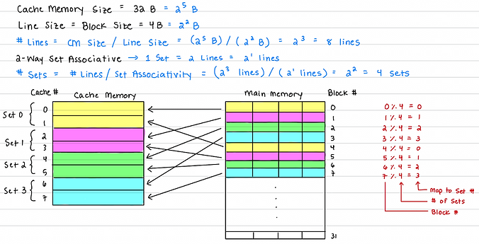
Here is an example of how the Main memory blocks get mapped to the Cache memory for 2-way associativity:

TASK:

The goal for this project is to implement a simulator using Python that functions like a Cache memory component. The Cache simulator will need to read addresses from an “addr_trace” file and check to see if they are stored in the Cache memory. It will be a Cache hit if it is found or a Cache miss if it is not found. Once all addresses have been read, we will need to display the total number of simulates addresses, total number of Cache hits, and Cache hit ratio. The simulator will need to work for the following parameters:

Cache Memory Size: 16KB, 32KB, 64KB, 128KB
Block Size: 16B, 32B, 64B, 128B
Associativity: Direct, 2-way, 4-way, 8-way, Fully
Replacement Policy: Least Recently Used (LRU), First In First Out (FIFO), Random

Miss Rate diagrams will also need to be provided.

DESIGN PROCESS:

To make the coding process simpler and easier to follow, I began by first creating a diagram (Figure 5) of the simulator to visualize what steps I need to take when implementing the design. The parameters will be entered on the terminal, which will be parsed in the Python code. Those parameters will determine the Physical Address (PA) split which are the Tag, Index, and Offset bits. Meanwhile, the addresses in the “addr_trace” file will be read and converted into binary. This will now allow us to obtain the needed information (address’s tag, index, and offset bits, associativity, and replacement policy) to begin checking the Cache Memory.

Figure 5: Cache Simulator Diagram.

Before proceeding with the design explanation, it is important to mention that the design will include a Cache memory table, a validation table, and a replacement tracker table. Whenever a value is stored in the Cache memory table, the validation table will store a ‘1’ in that same index to indicate that the value stored is valid. If there is no value stored in a line, then the validation table will store a ‘0’. This will allow us to keep track of how much memory is still available or when it is full. In a case where we are using set associativity and the Cache is full, we need to know which line we can replace. The replacement tracker table will solve that by storing a number for each line. The tracker will look at the number stored to determine which line has been the least frequently used or which was written first. That number will increment whenever the line is read or written. For example, if set 0 has 2 lines with stored data and we receive a Cache miss, we will need to write the new data into 1 of the 2 lines. To determine which line to overwrite, we will look at the replacement tracker table. The tracker, for example, will have the number 23 stored for line 1 and 24 for line 2. With this information, we can see that since line 1 has the smaller number, it was stored into the set first and has been there the longest. Therefore, the algorithm would select line 1 to replace and increment the number in the tracker to 25.

When the Cache memory is checked, it will search for the tag in the specified index from the PA. If the tag is there it will increment the Cache Hit Counter by 1 and update the replacement tracker. If the tag is not found, it will increment the Cache Miss Counter by 1. It will then use the Validation table to see if all the lines are full. If they are not, the new data will be written to the next available line, else it will refer to the replacement tracker and see which of the lines can be replaced. The new data will be written into the Cache and the replacement tracker updated. After all addresses have been read and determined whether it is a Cache hit or miss, the Hit Rate Ratio will be calculated and displayed in the terminal.

SIMULATION/VERIFICATION

The parameters that are entered in the terminal need to be written in the following order: [Cache_Size] [Block_Size] [Associativity] [Replacement Policy]. Below I have taken screenshots of the terminal after simulation. Figure 6 displays the Hit Ratio for LRU, FIFO, and Random for a 16KB Cache with 32B Blocks and 4-way associativity. Figure 7 shows the simulation results for Direct and Full Associativity.

Figure 6: a) LRU b) FIFO c) Random Simulation Results.

Figure 7: a) Direct and b) Full Associativity Simulation Results.

The graphs (Figures 8-10) below display the Cache Miss Rate for the 3 replacement policies in respect to all the Cache memory sizes, Block sizes, and Associativity.

Figure 8: Cache Memory Size Miss Rate.

Figure 9: Block Size Miss Rate.

Figure 10: Associativity Miss Rate.

The hardest task of the project was trying to relearn Python as I have not used the programming language in a long time. But after looking at a few Python guides and examples, I was able to easily pick it up and begin working on the project. I had initially planned to implement the project in Verilog since it is the language that I am the most familiar with but was not recommended. Besides that, I did not encounter any major many issues.

CONCLUSION:

This project is a great opportunity for students to further their understanding of Cache memory even more by seeing how different parameters can improve the Hit Ratio. Although learning the concepts in class are useful, being able to implement them in software ensures a full understanding. I found this project to be slightly challenging initially because I was not familiar with Python, therefore I had to take some time to learn and understand the syntax. But after some practice, I was able to begin programming the project. If I had more time on the project, I would have rewritten my code so that it could be more organized and efficient by using classes and a main function. As of right now, different sections of my code are only separated by comments. Overall, I enjoyed working on this project and believe it is an essential assignment because it helped me further my understanding of the Cache memory and regain my Python programming skills.